

Perhaps you’ve come across the paper From Local to Global: A GraphRAG Approach to Query-Focused Summarization, which is Microsoft Research’s take on Retrieval Augmented Generation (RAG) using knowledge graphs. Perhaps you felt like some sections in the paper were vague. Perhaps you wished the documentation more thoroughly explained how information gets retrieved from the graph. If that sounds like you, read on!
I’ve dug through the code, so you don’t have to, and in this article, I’ll describe each step of the GraphRAG process in detail. You’ll even learn a search method that the paper didn’t mention at all (Local Search).
What Is GraphRAG?
In one sentence, GraphRAG is an enhancement to retrieval-augmented generation that leverages graph structures.
There are different implementations of it, here we focus on Microsoft’s approach. It can be broken down into two main steps: Graph Creation (i.e. Indexing) and Querying (of which there are three possibilities: Local Search, Global Search and Drift Search).

Key GraphRAG steps: Graph creation and graph querying
Set-Up
The GraphRAG documentation walks you through project set-up. Once you initialize your workspace, you’ll find a configuration file (settings.yaml) in the ragtest directory.

Project structure
I’ve added the book Penitencia to the input folder. For this article, I’ve left the config file untouched to use the default settings and indexing method (IndexingMethod.Standard).
Graph Creation
To create the graph, run:
graphrag index --root ./ragtest
This triggers two key actions, Entity Extraction from Source Document(s) and Graph Partitioning into Communities, as defined in modules of the workflows directory of the GraphRAG project.

Modules implementing entity extraction and graph partitioning into communities. The numbers (yellow) show the order of execution.
Entity Extraction
1. In the create_base_text_units module, documents (in our case, the book Penitencia) are split into smaller chunks of N tokens.

The first five chunks of the book Penitencia. Each chunk is 1200 tokens long and has a unique ID.
2. In create_final_documents, a lookup table is created to map documents to their associated text units. Each row represents a document and since we are only working with one document, there is only one row.

Table showing all documents by their IDs. For each document, all the associated chunks (i.e. text units) are listed by their IDs.
3. In extract_graph, each chunk is analyzed using an LLM (from OpenAI) to extract entities and relationships guided by this prompt.
During this process, duplicate entities and relationships may appear. For example, the main character Jon is mentioned in 82 different text chunks, so he was extracted 82 times — once for each chunk.

Snapshot of the entity table. Entities are grouped by entity title and type. The entity Jon was extracted 82 times, as observable from the frequency column. The text_unit_ids and description columns contain a list of 82 IDs and descriptions, respectively, showing in which chunks Jon was identified and described from. By default, there are four entity types (Geo, Person, Event, and Organization).

Snapshot of the relationship table. Relationships are grouped by source and target entities. For Jon and Celia, the description and text_unit_ids columns contain lists with 14 entries each, revealing that these two characters had relationships identified in 14 distinct text chunks. The weight columns shows the sum of the LLM-assigned relationship strength (weight is not the number of connections between source and target nodes!).
An attempt at deduplication is made by grouping together entities based on their title and type, and grouping together relationships based on their source and target nodes. Then, the LLM is prompted to write a detailed description for each unique entity and unique relationship by analyzing the shorter descriptions from all occurrences (see prompt).

Snapshot of the entity table with the final entity description (composed from all extracted short descriptions).

Snapshot of the relationship table with the final relationship description (composed from all extracted short descriptions).
As you can see, deduplication is sometimes imperfect. Furthermore, GraphRAG does not handle entity disambiguation (e.g. Jon and Jon Márquez will be separate nodes despite referring to the same individual).
4. In finalize_graph, the NetworkX library is used to represent the entities and relationships as the nodes and edges of a graph, including structural information like node degree.

Snapshot of the final entity table where each entity represents a node in the graph. A node’s degree is the number of edges it has (i.e. the number of other nodes that it connects to).

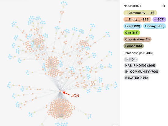
I find it helpful for understanding to actually see the graph, so I have visualized the result using Neo4j (notebook):

The book Penitencia visualized as a graph using Neo4j

The entity Jon and his relationships visualized using Neo4j

The relationship between Laura and Mario visualized as a graph edge using Neo4j
Graph Partitioning into Communities
5. In create_communities, the graph is partitioned into communities using the Leiden algorithm, a hierarchical clustering algorithm.
A community is a group of nodes that are more closely related to each other than to the rest of the graph. The hierarchical nature of the Leiden algorithm allows for communities of varying specificity to be detected, which is reflected in their level. The higher the level, the more specific the community (e.g. level 3 is quite specific, whereas level 0 is a root community and very generic).

If we visualize each community as a node, including the entities belonging to the community, we can make out clusters.

The Penitencia graph filtered for IN_COMMUNITY relationships reveals 15 root level communities (red circles)

Neo4j visualization of three hierarchically connected communities: Community 2 (Celia Gómez and the Tetuán Incident) — [parent of]→ Community 23 (Celia’s Desperation and Familial Violence) — [parent of]→ Community 42 (Celia’s Struggle with Laura). Rank is the LLM-assigned importance of the community from 1 (lowest importance) to 10 (highest importance).
6. In create_final_text_units, the text unit table from Step 1 has the entity IDs, relationship IDs and covariate IDs (if any) mapped to each text unit ID for easier lookup.

Covariates are essentially claims. For example, “Celia murdered her husband and child (suspected).” The LLM deduces them from the text units guided by this prompt. By default, covariates are not extracted.
7. In create_community_reports, the LLM writes a report for each community, detailing its main events or themes, and a summary of the report. The LLM is guided by this prompt and receives as context all the entities, relationships and claims from the community.

For large communities, the context string (which includes entities, relationships and, possibly, covariates) might exceed the max_input_length specified in the config file. If that happens, the algorithm has a method to reduce the amount of text in the context, involving Hierarch Substitution and, if necessary, Trimming.
In Hierarchal Substitution, the raw text from entities, relationships, claims is replaced by the community reports of sub-communities.
For example, suppose Community C (level 0) has the sub-communities S1 and S2 (both level 1). Community S1 is larger in size (has more entities) than S2. Given this situation, all entities, relationships, and claims in C which are also in S1 are replaced by the community report of S1. This prioritizes the biggest reduction in token count. If context length still exceeds max_input_length after this change, then S2 is used to replace relevant entities and relationships in C.
If after hierarchal substitution, the context is still too long (or the community had no sub-communities to begin with), then the context string needs Trimming — less relevant data is simply excluded. Entities and relationships are sorted by their node degrees and combined degrees, respectively, and those with the lowest values are removed.
Ultimately, the LLM uses the provided context string to generate findings about the community (a list of 5–10 key insights) and a summary. These are joined to form the community report.


8. Finally, in generate_embeddings, embeddings for all text units, entity descriptions, and full_content texts (community title + community summary + community report + rank + rating explanation) are created using the Open AI embedding model specified in the config. The vector embeddings allow for efficient semantic searching of the graph based on a user query, which will be necessary during Local and Global Search.
